
Benchmark study of approaches to estimate probability of default in the context of climate risk
Perspectives
Benchmark study of approaches to estimate probability of default in the context of climate risk
Tue 27 Jul 2021
Recently, initiatives to tackle climate-related and environmental risks in the financial services industry have begun across the world. These initiatives followed the adoption of the United Nations Paris Agreement on climate change, the 2030 agenda for Sustainable Development and the European Green Deal.
Stress testing and scenario analysis are a common framework proposed by different regulatory and supervisory bodies across various countries to assess the impact of climate-related risks on the financial system. Countries like the United Kingdom and France, having started working on pilot climate stress test exercises, are leading by example. However, no consensus regarding the best methodology to use in this context has been reached as of today.
In this article, Mazars presents the results obtained by implementing two methodological approaches to estimate the sectoral probability of default (PD) parameters in the context of climate risk stress testing:
- The first methodology studied was developed as part of the UN Environmental Programme (UNEP) Finance Initiative when piloting the implementation of recommendations outlined by Task Force on Climate-related Financial Disclosures (TCFD)[1]; and
- the second corresponds to the approach followed by the Autorité de Contrôle Prudentiel et de Résolution (ACPR) in its 2020 climate risk stress test pilot exercise[2].
Common basis of the two approaches
Both approaches are built upon a well-established PD methodology, known as the Merton Framework, where the default dynamics are captured via macroeconomic and financial risk drivers. This allows one to project the expected default rate according to the anticipated movements of these risk drivers. The Merton model has been widely used in the industry to derive the IFRS 9 forward-looking and point in time PDs and perform stress testing.
With this foundation, the two approaches differ in the way the framework has been adapted for climate stress testing. In particular, the approaches differ in the mode of incorporation of climate risk factors into the PD calculations. The results obtained by Mazars show that these two distinct approaches can yield similar results.
Sectoral sensitivity approach
In this approach, climate variables and their respective sensitivity coefficients -estimated using a scorecard – are added into the sectoral PD Merton models. As previously mentioned, the method was developed by the UNEP, and we refer to it as the “sensitivity approach” throughout this article.
This approach has two clear advantages:
- it requires few additional inputs; and,
- one can leverage the work performed by the UNEP when determining the hierarchy of the sensitivities (i.e. which sectors have a high climate risk impact vs low).
However, a key drawback is the lack of guidance or references for the level of the sensitivities, so the determination of these inputs is based on expert judgement.
Sectoral approach
The French regulator, the ACPR, produced a set of sectoral Gross Value Added (GVA) forecasts and existing leveraged models from banks when building its climate risk stress testing framework. Climate PD forecasts were produced using the sectoral forecasts given by the ACPR along with either the bank’s pre-existing models or with newly developed models. It is worth noting that when the bank’s PD models did not include GDP as a default risk driver, new models were developed to add it. This variable was necessary to produce forecasts with the sectoral granularity required for the climate risk stress testing assessment. Similarly, the BoE produced a set of sectoral GVA forecasts for its 2021 Climate Biennial Exploratory Scenario (CBES), accounting for different economic sectors’ varying degrees of exposure to climate risks.
This approach has three advantages:
- the work performed by the ACPR can be used as a reference;
- generally, results can be generated with slight modifications to existing models; and
- the model does not introduce additional parameters.
On the other hand, the disadvantages include:
- a strong modelling assumption: “models are still pertinent with sectoral data”; and,
- the requirement of sectoral macro-economic forecasts.
Our study
Mazars implemented both methodologies in an attempt to understand whether the methodologies yield consistent results. In practice, our study consisted of the following steps:
Step 1. Calibrating a PD model to the historical default rate series of the global corporates segment, which, by design, included a GDP variable.
Step 2. Applying the PD model (obtained in step 1) to the ACPR sectoral forecasts to derive results from the sectoral approach.
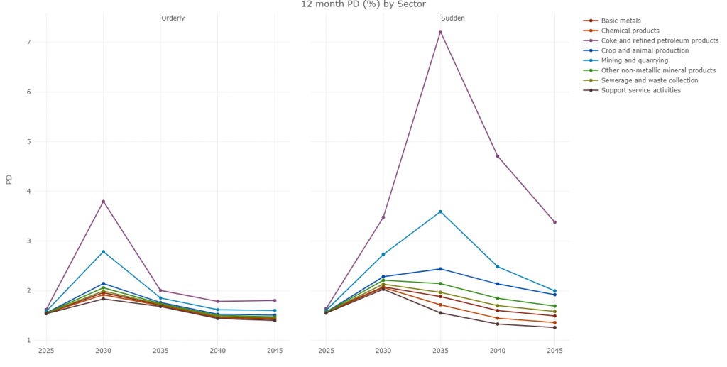
Figure 1. Forecast of 12-month PD by sector for two ACPR scenarios
Figure 1 illustrates the 12-month PD forecast at each reporting date for two ACPR scenarios: orderly and sudden. To provide some context, the ACPR orderly scenario reflects the French roadmap designed to fulfil the commitments made under the Paris Agreement. On the other hand, the sudden and delayed scenarios consist of a sharp increase in the carbon price, the latter starting only in 2030.
As expected, one can see that the risk parameter (i.e. PD) increases with the “severity” of the scenario. A similar fact can be highlighted for the segments: a higher PD is observed for those segments expected to have stronger negative impacts from climate change.
Step 3. Calibrating the sensitivities (in the sensitivity approach) of each sector to climate variables. The sensitivity for each sector was estimated such that the difference in 12-month PD at each calculation date between the results from the sensitivity approach and the sectoral approach is minimised.
Mazars selected the annual difference in carbon price as the climate variable. Other transformations of carbon price were analysed but won’t be considered in this article because the results obtained were consistent with those discussed here.
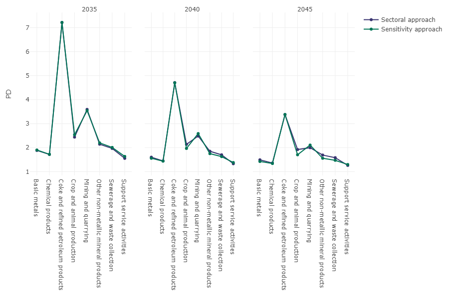
Figure 2 illustrates the 12-month PD by sector at three reporting dates (2035, 2040 and 2045) utilising the two alternative approaches.

Figure 2. 12-month PD in 2035, 2040 and 2045 for the sudden scenario using the difference in the carbon price
The left graph in Figure 2 illustrates the 12-month PD by sector for the sudden scenario as at 2035 and shows that the two approaches yield consistent results for five out of the seven sectors analysed. There is, however, a significant difference when comparing the two most sensitive sectors: coke and refined petroleum and mining and quarrying.
On the other hand, for the 2040 reporting date, the results show convergence for all the sectors (refer to the graph in the centre in Figure 2). Small discrepancies were observed for the 2045 reporting date (refer to the right graph in Figure 2). These can be explained by differences in the information carried by the selected climate risk variables (GVA forecasts vs difference in carbon price).
In an attempt to reduce the discrepancies between the two approaches, an additional analysis was performed by implying a climate factor from the GVA forecast of the most affected sector (i.e. coke and refined petroleum products) relative to the GDP forecast. We will refer to this variable as the ACPR implied climate factor and, for each year, define it as follows:

where  and
and  are the annual differences of each variable respectively.
The results obtained using the ACPR implied climate factor for 2035, 2040 and 2045 are shown in Figure 3.
The sensitivity approach results fit the sectoral GVA approach results almost perfectly, particularly for the coke and refined petroleum products sector. The latter behaviour was expected as the ACPR implied climate factor was built using the GVA forecasts for this sector. We observed slight discrepancies for some sectors in the sudden and delayed scenarios and when looking at all reporting dates.
Step 4. Analysis of the results.
Table 1 summarises the results of the calibrations performed in step 3, along with the ratio of the sectoral GVA forecast from the ACPR divided by the GDP forecast (sector independent). These ratios are used to benchmark our results as they represent the ACPR expected climate impacts for each of the sectors.
Furthermore, the values in Table 1 have been colour-coded such that the sectors that are highly impacted by the climate risk are highlighted in red, and those that are less impacted are highlighted in green.
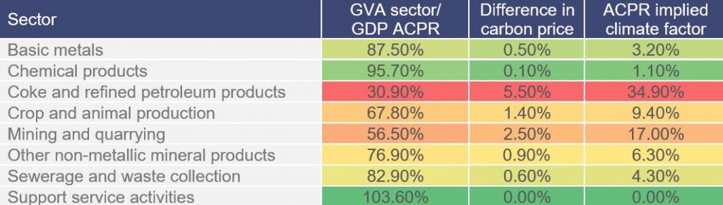
The results obtained when calibrating the sensitivities with both variables (difference in carbon price and the ACPR implied climate factor) are consistent. With both methods, the most impacted sector was coke and refined petroleum products, followed by mining and quarrying, and the least impacted sector was support service activities. The same conclusion is reached when comparing the sensitivities with the GVA/GDP ratios[3].
Finally, we compared our results with the scorecard ratings provided in the UNEP/TCFD study “Beyond the Horizon”[4]. Table 2 outlines the mapping applied and the associated UNEP/TCFD ratings by sector.
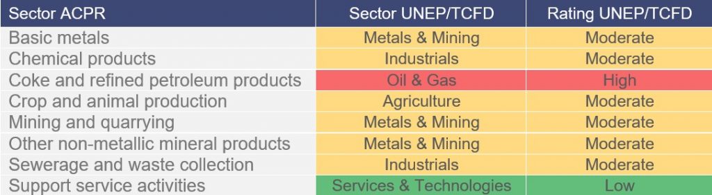
Overall, the results presented in Table 1 appear to be consistent with the ratings summarised in Table 2 except for the Metals & Mining sector. The UNEP rated this sector as “Moderate”, whereas the GDP ratios from ACPR indicate the segment is treated as “Highly Moderate”. Notice that there is a clear difference between the ratios of this sector (orange rows in Table 1) and the rest of the sectors rated as “Moderate” (yellow rows in Table 2). The discrepancy could be explained by differences in the segmentation approaches of the two sources.
Conclusion
Based on the results obtained, we conclude that both sensitivity and sectoral approaches can yield equivalent results, particularly when both methods use the same climate risk information to project PDs.
[1] Extending Our Horizons by J. Colas, I. Khaykin, A. Pyanet and J. Westheim, April 2018, available here.
[2] Analysis and synthesis no. 122: The main results of the 2020 climate pilot exercise, by ACPR, May 2021, available here.
[3] These ratios are estimated as the average ratio across scenarios for each sector for the 2050 forecast. For example, we divided the basic metals GVA 2050 forecast of the accelerated scenario by the GDP 2050 forecast for the accelerated scenario respectively, and then average them to consider the three scenarios.
[4] Beyond the horizon: New Tools and Frameworks for transition risk assessments from UNEP FI’s TCFD Banking Programme, by D. Carling and R. Fischer, September 2020, available here.
Want to get notified when new blog posts are published?
Subscribe 
Christophe Bonnefoy Partner - Paris

The FED announced a pilot climate scenario analysis exercise for early 2023
The Federal Reserve Board (FED) will commence its first bottom-up climate scenario analysis exercise at the beginning of 2023, as announced on 29 September. The exercise will be exploratory in nature and will not result in extra capital requirements. The list of designated participants consists of six of the largest U.S. banks, i.e., Bank of […]

Results of the ECB 2022 climate risk stress test
The first supervisory climate risk stress test (2022 CST) conducted by the European Central Bank (ECB) has concluded with official results and findings made public on 8 July 2022. The exercise has complemented the broader ECB’s agenda to assess the readiness of banks in Europe to manage climate-related and environmental risks. The 2022 CST was […]

Our top risks for financial services firms in 2024
We have identified and ranked the key risks for financial services business leaders in 2024 based on market research, regulatory insights as well as our assessment of the current difficulties facing firms. We discuss in this article the key takeaways for you and your organisation. A more detailed assessment can be found here, which contains […]

How the insurance sector is meeting ESG challenges
This article is part of the series covering the impact of sustainable finance on the insurance sector. Read further:Part 1: Assessing the impact of sustainable finance on insurance entitiesPart 3: Developing a toolkit for responsible investment decisions When taking environmental, social, and long-term asset portfolio issues into consideration, insurance companies must assess the specific risks […]

Embarking on an ambitious common climate framework
As part of the European Green Deal, the European Union intends to encourage green investments and prioritise the revision of the Non-Financial Reporting Directive (NFRD). The European or Green Taxonomy, which sets out a precise classification of sustainable activities with the strategic objective of redirecting capital flows towards those activities from 2022, is a result […]

Sustainability and climate risk: what can banks expect?
The growing importance of sustainability issues and the role of credit institutions in financing transformation places climate and environmental risks at the core of regulatory and supervisory scrutiny today. For some years now, the Network for Greening the Financial System (NGFS), comprising central banks and national supervisory authorities, has been working to enhance sustainability and […]

The FSOC weighs in on climate risk
The Financial Stability Oversight Council (FSOC) was established under the Dodd-Frank Wall Street Reform and Consumer Protection Act as a result of the 2007-2008 US financial crisis. A first of its kind, the 15-member council is tasked primarily with identifying growing systemic risks to US financial stability and proposing coordinated regulatory responses to both preempt […]

First ACPR climate stress test pilot exercise results
Climate change introduces considerable economic challenges. On the one hand, financial institutions must contribute to the transition to a low-carbon and balanced economy to effectively combat global warming. On the other hand, the financial sector is exposed to climate-related and environmental risks and therefore needs to implement appropriate risk management practices within a financial stability […]

The Single Supervisory Mechanism: Post-pandemic actions and expectations
On 30 July, the European Central Bank unveiled the 2021 supervisory stress test results, which demonstrated that the region’s banking system is resilient in an unfavourable environment. The Common Equity Tier 1 (CET1) ratio has fallen 5.2% to 9.9% under the 3-year adverse scenario, while under the baseline scenario the CET1 ratio will reach 15.8% […]

ESG investing: Three risks to consider
The continued popularity of funds with an environmental, social and governance (ESG) focus has put global ESG assets on track to exceed $53tn by 2025, up from nearly $38tn at the end of 20201. As growth continues, expectations for effective compliance policies and controls in place are expected to become more rigorous as political and […]

ESG investing: From buzzword to mainstream
A growing interest in environmental, social and governance (ESG) issues is driving record inflows into the ESG-led investment sector. During 2020, sustainable funds available to European investors attracted net inflows of €233bn1, which saw assets under management hit the $1.1tn milestone, accounting for almost 10% of total European fund assets. A similar growth story in […]

EBA: draft technical standards on Pillar 3 disclosures of ESG risks
On 1 March 2021, the European Banking Authority (EBA) launched a public consultation on draft implementing technical standards (ITS) for Pillar 3 disclosures of environmental, social and governance (ESG) risks, under its capital requirements regulation (CRR) mandate. The consultation will end on 1 June 2021. Large banking institutions with securities traded on a regulated market […]

Managing an increase in bank credit risk
While 2020 went relatively smoothly for the banking sector, uncertainties remain on the potential effects of Covid-19 on the real economy. Any negative impact could lead to heavy losses for the sector, especially when support measures are gradually phased out. These measures have not only contained the anticipated increase in credit risks, but have also […]

The impact of credit risk on 2021 stress tests
On 13 November 2020, the EBA published the final methodological note for the 2021 EU-wide stress-testing exercise. The aim of the stress tests is to assess the resilience of financial institutions to adverse economic and financial developments, in particular in the event of an increase in credit risk due to the default of the borrower. […]

EBA discussion paper on the management and supervision of ESG risks
European sustainable finance regulations evolved considerably in 2020, and the European Banking Authority (EBA) is continuing this trend into 2021. It recently published a discussion paper assessing the potential inclusion of Environmental, Social and Governance (ESG) risks in the supervisory review and evaluation process (SREP) performed by national competent authorities (NCAs)[1]. What firms need to […]

Developing a toolkit for responsible investment decisions
This article is part of the series covering the impact of sustainable finance on the insurance sector. Read further:Part 1: Assessing the impact of sustainable finance on insurance entitiesPart 2: How the insurance sector is meeting ESG challenges Clarity of information provided to various stakeholders is a growing issue for financial organisations. Despite the efforts […]

Assessing the impact of sustainable finance on insurance entities
This article is part of the series covering the impact of sustainable finance on the insurance sector. Read further:Part 2: How the insurance sector is meeting ESG challengesPart 3: Developing a toolkit for responsible investment decisions Amid a global pandemic and a rising threat of climate change, today’s society expects financial organisations to uphold strong […]

Eurofi financial summit addresses EU’s ecological and digital transition
As a setting for exchange between European Union (EU) economic and financial regulators and senior financial sector executives from the industry, one of the world’s largest financial services conferences, Eurofi, took place in Paris in February. Established in 2000, the Eurofi meetings occur bi-annually* alongside the Economic and Financial Affairs Council configuration (ECOFIN) meetings. The […]

A looming climate crisis?
Persistant negative interest rates, the inherent risk of a trade war between China and the United States, fears of a recession… all worrying signs of an imminent new crisis. However, the real question is not if but when the next crisis will hit. More than ten years after the financial and sovereign debt crisis, it […]

Ultimate Forward Rate (UFR): Why we are seeing a change to the rate curve
On 6 February 2018, EIOPA published its latest risk-free interest rate curve to be taken into account for the purposes of Solvency II calculations. Based on calculations for January 2018, the curve is slightly different from previously published curves. This is reflecting significant changes in the long-term expectations of interest rates in recent years which calculates […]

SFCR: Review of narrative reports, good practices and EIOPA recommendations
The Solvency II Directive increases the requirements for transparency vis-à-vis both the regulatory authorities and the stakeholders, including policyholders, financial analysts and investors. In this context, insurance undertakings and groups were, for the first time, required to publish a narrative report no later than 19 May 2017, known as the Solvency and Financial Condition Report […]

Overview of the US Stress Test Scenarios Vs. the European Scenarios
On February 1, 2018, just one day after the European Banking Authority (EBA) officially kicked off its EU-wide stress test exercise, the Federal Reserve Board (FRB) released the applicable scenarios for its own US stress test. 2018 US Stress Test Scenarios Overview The annual stress test exercise is required by a provision of the Comprehensive […]

European banks are better armed against macro-economic shocks
On Friday 2 November, as expected, the European Banking Authority (EBA) published the results of the 2018 EU wide stress tests on European banks’ solvency in the event of macro-economic shocks. This was the fourth exercise of the now-biannual testing which has been carried out on European Union banks. Despite more severe tests than in […]

Climate change: a threat to the stability of the financial services
With rising global temperatures[1] comes an ever-growing pressure on the financial services sector to respond and prepare for the far-reaching effects of climate change. The impacts upon the sector are already being felt – extreme weather events are creating significant losses for insurers and credit risks for banks, and pressures on businesses to demonstrate sustainable […]

Climate change: the Bank of England’s commitments
In 2018, the Bank of England (the “BoE”) set up a project called “Future of Finance” aimed at anticipating the upcoming changes in financial services for the next decade, and the impact of these changes for market participants, customers and regulators. This research was led by Huw van Steenis, Senior Adviser to the Governor, and […]

How will COVID-19 affect the financial regulatory response to climate change?
At first glance, regulatory authorities appear to have deprioritised the issue of climate change. However, a closer look would suggest otherwise and climate change in reality remains a key long-term priority of national and European regulators. In some areas, regulatory action on climate change has been delayed Central banks around the world have taken steps […]

Injecting noise into the discussion
Michael Lennard, Chief of International Tax Cooperation and Trade in the Financing for Sustainable Development Office (FfDO) of the United Nations, examines the role of tax toolkits for developing countries from a personal perspective. The Platform for Collaboration on Tax (PCT) involving the UN, OECD, IMF and the World Bank, is certainly a good example […]

How banks can demonstrate responsible banking during the pandemic
What is the purpose of a bank? Does it have a responsibility to society at large, over and above its duties to its shareholders, customers and employees? The purpose of banks – to make a profit or be socially useful? What is the purpose of a bank? Does it have a responsibility to society at […]

Federal reserve board publishes 2020 stress testing results and additional sensitivity analysis
The Federal Reserve Board released stress test results for DFAST 2020 including additional sensitivity analysis, considering the COVID19 outbreak, to assess the resiliency of large banks under three hypothetical recessions, or downside scenarios, that could result from the coronavirus event. Furthermore, the Board provides guidance for large banks to maintain resiliency during economic uncertainties from […]

Bank stress tests – the post Covid agenda
In the early 1990s, stress tests became a popular internal tool for international banks to examine risks and gain a better understanding of threats to the institutions’ balance sheet. From there, the Basel Accord was amended in the mid- ’90s and required banks and investment firms to conduct stress tests. However, these were more internal […]

Addressing the challenges of the new sustainable finance regulations
As the world gears up for the transition to net-zero, the European Union is setting ambitious targets with respect to its own environmental footprint. For instance, by 2030 the EU is looking to reduce European greenhouse gas emissions by at least 55% compared to 1990 levels; increase the share of renewables within Europe’s total energy […]

2021 Stress testing the UK banking system: the Bank of England’s approach
March 2020 marked the first time – since its inception in 2014 – that the Bank of England (BoE) cancelled its annual stress tests for the UK’s biggest lenders. Instead, they undertook a desktop analysis of the UK banking sector resilience. In late 2020, the Financial Policy Committee (FPC) judged that most banks have capital […]

Building a more inclusive tax model
Michael Lennard, Chief of International Tax Cooperation and Trade in the Financing for Sustainable Development Office (FSDO) of the United Nations, discusses, from a personal perspective, a range of key issues on the UN’s approach to transfer pricing. In 2019 the United Nations Tax Committee issued draft guidance on financial transactions. It was finalized in […]

Banks need to step up efforts on climate and environmental risk disclosures
In March 2022, the European Central Bank (ECB) published its second snapshot of climate-related and environmental risk disclosure levels among significant institutions under its direct supervision. In line with the results of the first snapshot published in November 2020 – regarded as the baseline measurement – none of the institutions in scope for this second […]

France steps up sustainable transformation with mission-led business law
France’s innovative and incentivising Action Plan for Business Growth and Transformation (PACTE) law lays the legal foundations for corporate social responsibility. With more than 400 companies established as “sociétés à mission” – mission-led businesses – by the end of 2021, this new scheme is an undeniable success. The number of mission-led companies has doubled in […]

Sustainable finance regulations signal a sea change for insurance sector
The European Green Deal aims to achieve climate neutrality by 2050 and create a modern, competitive and resource-efficient economy. To meet its objectives, the European Commission has begun to restructure the non-financial reporting requirements for companies. Although some of the requirements were partially implemented in 2021, this is only the beginning of a real sea […]

IIF annual membership meeting: building resilience amid turbulence and transformation
The IIF Annual Membership meeting is a setting for insights and perspectives from global financial regulators and senior financial sector executives on topical economic and regulatory issues. Being a forum with global coverage means that it is a valuable setting for picking up future economic and regulatory directions. A packed agenda under the theme of Building […]

The European Central Bank’s priorities for 2024: where do we stand after the first quarter?
The European Central Bank (ECB) issued the SSM supervisory priorities for the 2024-2026 cycle on 19 December 2023. They sum up what institutions under the direct supervision of the ECB should expect in terms of areas of supervision, in 2024 notably, and allow firms to prepare themselves for forthcoming onsite inspections or thematic reviews. Please […]

Unveiling the European Central Bank’s strategy: data, scenarios and models
In January 2024, the European Central Bank (ECB) published its Climate and Nature Plan for 2024-2025. This plan aims to: This plan underscores those financial risks stemming from climate change remain a key area of attention for the ECB. The ECB will continue working on several topics including stress testing, scenarios and climate-related data, and […]

How banks and insurers have progressed in embedding sustainability into their businesses
In late 2023, and to coincide with COP 28, Mazars published its latest Sustainability practices survey on the progress banks and insurers have made in embedding sustainability into their businesses, our most comprehensive and information-rich report to date covering 404 executives in banks and insurance companies in 16 countries Despite sustainability being in the limelight […]

Assessing materiality and verification of sustainability disclosures
In environmental, social and governance (ESG) reporting, materiality is crucial for enhancing transparency and accountability in sustainability and climate-related disclosures. Importantly, it helps identify and report on matters that are deemed significant, emphasizing their relevance to stakeholders. Materiality comes in various forms. Financial materiality focuses on sustainability issues impacting financial performance, aligning with annual financial […]

What’s driving financial firms’ sustainability strategies?
To adapt to the swiftly evolving regulatory landscape and meet stakeholders’ expectations, financial firms are increasingly formulating sustainability strategies to address environmental, social and governance (ESG) factors. Notably, emissions reduction and the pursuit of net-zero targets have become central elements of ESG strategies for many financial firms, according to the latest Mazars’ survey Sustainability practices stocktake: […]

Mitigating the financial impacts of climate-related risks
The integration of environmental, social and governance (ESG) considerations into strategic planning is increasingly becoming a common practice among financial services firms. However, climate-related risks can also serve as drivers of financial risk for institutions. These risks can manifest through various transmission channels, translating climate and environmental (C&E) risks into more conventional categories such as […]

How are financial institutions reflecting C&E considerations in risk appetite statements?
There is growing pressure for banks and insurers to incorporate C&E factors in their risk management frameworks (RMF). As a practice, it gives the ability to set clear thresholds for the climate impacts banks and insurers are willing and able to absorb. By establishing these thresholds, firms can effectively monitor their exposure to C&E risks, […]

Adapting governance to spearhead sustainability more effectively
There are increasing regulatory expectations globally for financial institutions to disclose and demonstrate how sustainability-related responsibilities are allocated within the organisation. In this respect, the increasing global trend towards mandatory sustainability disclosure frameworks continues to underscore the significant role that the finance function is anticipated to assume in sustainability. It’s a trend reflected in Mazars’ […]

The insurance industry in flux: what changes are currently unfolding?
The regulatory requirements for insurance companies are becoming increasingly complex. In this interview, Marc Böhlhoff and Thomas Volkmer, Partners at Mazars in Germany, discuss the impact of this change on the industry and delve into what it means for the operations of auditing and consulting firms. Mr. Volkmer, the insurance industry is undergoing rapid change. What […]

How financial institutions can move sustainability reporting to real-world application
The increased demand for sustainable finance shows that awareness of environmental, social and governance (ESG) issues is generally high among financial institutions. Indeed, for many of the larger players subject to the EU’s Non-Financial Reporting Directive (NFRD), there has been a requirement to include ESG information in annual reports for some time. Others have incorporated […]

Managing tomorrow’s banking risks
While the banking sector has shown resilience over recent years, the economic environment and geopolitical situation remain tense. So, what does this mean for risks to the banking sector? More specifically, what is the impact on capital requirements for banks with the implementation of the Capital Requirements Regulation (CRR3) and the Capital Requirements Directive (CRD6), […]

European green taxonomy eligibility ratios in the banking sector
The implementation of the European Union’s ‘Taxonomy’ regulation, which integrates two climate objectives, was carried out on 1 January 2022 through the ‘Climate’ Delegated Act released in April 2021. In line with this, the banking sector has been provided with corresponding regulations, allowing banks to measure the portion of their financing dedicated to sustainable economic […]

Transitioning to greener practices in the real estate sector
In 2022, the European Union implemented the green taxonomy for the second year, requiring companies to disclose indicators related to climate objectives. The green taxonomy aims to guide capital investment towards environmentally sustainable activities, making companies assess their alignment with the EU’s sustainable transition and enabling financial institutions to prioritise funding for projects contributing the […]

EUROFI financial forum: strengthening economic union and European competitiveness
The Eurofi financial forum is a setting for exchanges between European Union (EU) economic and financial regulators and senior financial sector executives from the industry. It occurs bi-annually alongside the Economic and Financial Affairs Council configuration (ECOFIN) meetings. This summary takes stock of the Eurofi discussions, as well as recent publications by the EU Commission […]
Our top risks for financial services firms in 2024
We have identified and ranked the key risks for financial services business leaders in 2024 based on market research, regulatory insights as well as our assessment of the current difficulties facing firms. We also highlight the changes in risk rankings compared to last year, justified by global events and new regulations that have surfaced in […]

Asset managers and ESG implementation: turning regulatory and operational compliance into commercial opportunities
ESG-related regulatory requirements, and scrutiny, show no signs of abating. Asset managers have a pivotal role in financing the transition towards low-carbon economic systems. Hence, governments have introduced several ESG-related regulatory requirements that apply to asset managers. Some examples of these are the Sustainable Finance Disclosure Regulation (SFDR) in the EU and the mandatory disclosures […]

Sustainable finance series: Why does sustainable finance matter?
The momentum towards a low-carbon economic system is only set to grow. Financial services firms are pivotal actors in the transition; consequently, increasing demands are being put on them to demonstrate their sustainable finance activities and credentials. This blog explains what sustainable finance is and why it matters to financial services firms. What is Sustainable […]

Sustainable finance series: Driving credible ESG actions
Implementing credible environmental, social and governance (ESG) actions requires successful enablers. So how can firms identify these enablers and, crucially, remove barriers to implementation? If we take our latest C-Suite Sustainability Barometer, we can see that out of the over 1,100 businesses accounted for in the survey, 75% are planning to increase their investment in […]

Climate change valuation adjustment: introducing a climate change scenario extrapolation to long dated CDS curve
The global climate crisis has triggered the financial sphere to address the way in which it conducts business. Climate risk consideration is currently growing in the banking industry but should also be considered by banks in the Credit Valuation Adjustment (CVA) when pricing derivatives. The credit risk for long dated derivatives (beyond 10 years), reflected […]

The Fed shares instructions on its first pilot climate scenario analysis exercise
The Federal Reserve Board (Fed) has shared instructions on its pilot climate scenario analysis exercise (CSA). Six of the largest U.S. banks, i.e., Bank of America, Citigroup, Goldman Sachs, JPMorgan Chase, Morgan Stanley, and Wells Fargo are participating in the exercise and are requested to submit their results along with documentation by July 31, 2023. […]

Why ESG-linked features impact financial assets classification under IFRS?
In our last article on sustainability-linked financing, we highlighted the accounting issues related to these contracts that are currently being debated between stakeholders. The most critical issue is the classification of loans or bonds that reference the borrower or issuer’s environmental, social and governance (ESG) key performance indicators (KPIs) on the balance sheet of lenders […]

COP27: stepping up implementation and the role of finance
A lot of attention at COP27 was focused on the likelihood of keeping global warming to 1.5 °C, in line with the goals of the 2015 Paris Climate Agreement. The consensus was that we are in real danger of falling off track. Few nations revised their nationally determined contributions to reduce their carbon footprint compared […]

Results of the ECB 2022 thematic review on climate-related and environmental risks
The European Central Bank (ECB) has expressed a significant supervisory concern surrounding more than half of supervised banks in terms of the progress made on fulfilling the expectations specified in the Guide on climate-related and environmental risks. The ECB recently concluded its 2022 thematic review of the banking sector’s alignment with supervisory expectations. This review […]

EBA considers bottom-up stress testing with top-down elements
The European Banking Authority (EBA) is tasked, in cooperation with the European Systematic Risk Board (ESRB), to initiate and coordinate biennial EU-wide stress testing exercises to assess the resilience of institutions to adverse market developments. The objective is to provide supervisors, banks, and other market participants with a common analytical framework to consistently compare and […]

IFRS series on sustainability-linked financing
As environmental, social and governance concerns are becoming more and more prevalent, sustainable finance is now under the spotlight. The financial sector has a key role to play in achieving the ESG transition. One of the levies developed by the financial industry is to propose new kinds of financing that promote ESG practices and projects […]

Green taxonomy trends facing the real estate sector
The European Union (EU) has taken the first step in directing capital investments toward so-called sustainable activities with the introduction of the Green Taxonomy on 1 January 2022. For the real estate sector, the objective is to measure the share of eligible activities contributing to the first two climate objectives – the mitigation of climate […]

Reliable information key to the insurance sector’s ability to apply Green Taxonomy
The objective of the European Union’s Taxonomy regulation, in force since 1 January 2022, is twofold for the insurance and reinsurance sector. First, to measure the share of investments devoted to financing economic activities eligible for the taxonomy, known as the Investment Ratio. Second, to measure the share of gross premiums written in eligible non-life […]

Banks grapple with GAR objectives
In force since 1 January 2022, the European Union’s Taxonomy regulation aims to support the market for green finance. More specifically, greater transparency in the market will help prevent greenwashing by providing information to investors about the environmental performance of assets and economic activities of financial and non-financial information. For the banking sector, the target […]

How to address climate risk in the banking prudential framework
Climate change is now firmly in the focus of prudential regulators and supervisors across the globe. Against this background, the European Banking Authority (EBA) is mandated to assess whether a dedicated prudential treatment of exposures related to assets or activities associated substantially with environmental and social objectives would be justified. Based on its findings, the […]

Overview of US stress tests and CCAR’s results 2016
The Federal Reserve disclosed the results of its annual supervisory stress tests and CCAR (Comprehensive Capital Analysis and Review) respectively on 23 and 29 June 2016. In a combined exercise which has been running since the financial crisis, 33 US Bank Holding Companies (BHCs) were tested, including US-based banks and the American units of big […]